Moderated APIM: Hahn, Binnewies, & Dormann (2014)

Replicating the children × partner WNC interaction

The headline result of Hahn, Binnewies, & Dormann (2014, Journal of Vocational Behavior) is that the presence of children in a household moderates the partner crossover effect of work–nonwork conflict on relationship satisfaction. Couples with children buffer the negative crossover; couples without children show the full negative effect.

This tutorial replicates that finding with the simulated dyad_data dataset, using both multilevel and SEM specifications. The DGP has a small but detectable interaction (int_child_pwnc = +0.10) — your likelihood ratio tests should recover it.

Setup

Code

library(lme4)
library(lmerTest)
library(lavaan)
library(dplyr)
library(interactions)

load("../../../data/dyad_data.RData")

cat("Dyads with children:    ", sum(ddw$has_children == 1), "of", nrow(ddw), "\n")

Dyads with children:     37 of 100

Code

cat("Dyads without children: ", sum(ddw$has_children == 0), "of", nrow(ddw), "\n")

Dyads without children:  63 of 100

MLM specification

The baseline APIM (no moderation) is the same as the indistinguishable tutorial.

Code

model_base <- lmer(
  satisfaction ~ wnc + partner_wnc + recovery + partner_recovery +
    has_children + dual_earner + (1 | dyad_id),
  data = ddl
)

summary(model_base)

Linear mixed model fit by REML. t-tests use Satterthwaite's method [
lmerModLmerTest]
Formula: satisfaction ~ wnc + partner_wnc + recovery + partner_recovery +  
    has_children + dual_earner + (1 | dyad_id)
   Data: ddl

REML criterion at convergence: 289.1

Scaled residuals: 
     Min       1Q   Median       3Q      Max 
-2.38505 -0.66160 -0.03835  0.58461  2.75274 

Random effects:
 Groups   Name        Variance Std.Dev.
 dyad_id  (Intercept) 0.03146  0.1774  
 Residual             0.19191  0.4381  
Number of obs: 200, groups:  dyad_id, 100

Fixed effects:
                  Estimate Std. Error        df t value Pr(>|t|)    
(Intercept)        4.82397    0.17008  95.00000  28.362  < 2e-16 ***
wnc               -0.25597    0.04024 176.98929  -6.362 1.65e-09 ***
partner_wnc       -0.17794    0.04024 176.98929  -4.422 1.70e-05 ***
recovery           0.22614    0.03862 191.89949   5.855 2.03e-08 ***
partner_recovery   0.12475    0.03862 191.89949   3.230 0.001456 ** 
has_children       0.02622    0.07957  95.00000   0.330 0.742436    
dual_earner        0.30471    0.07959  95.00000   3.828 0.000231 ***
---
Signif. codes:  0 '***' 0.001 '**' 0.01 '*' 0.05 '.' 0.1 ' ' 1

Correlation of Fixed Effects:
            (Intr) wnc    prtnr_w recvry prtnr_r hs_chl
wnc         -0.171                                     
partner_wnc -0.171 -0.316                              
recovery    -0.611  0.309 -0.070                       
prtnr_rcvry -0.611 -0.070  0.309  -0.091               
has_childrn -0.069 -0.215 -0.215  -0.064 -0.064        
dual_earner -0.212  0.067  0.067  -0.083 -0.083  -0.008

The moderated model adds the two interaction terms: partner WNC × children, and actor WNC × children.

Code

model_mod <- lmer(
  satisfaction ~ wnc + partner_wnc + recovery + partner_recovery +
    has_children + dual_earner +
    partner_wnc:has_children + wnc:has_children +
    (1 | dyad_id),
  data = ddl
)

summary(model_mod)

Linear mixed model fit by REML. t-tests use Satterthwaite's method [
lmerModLmerTest]
Formula: satisfaction ~ wnc + partner_wnc + recovery + partner_recovery +  
    has_children + dual_earner + partner_wnc:has_children + wnc:has_children +  
    (1 | dyad_id)
   Data: ddl

REML criterion at convergence: 289

Scaled residuals: 
     Min       1Q   Median       3Q      Max 
-2.33706 -0.70526 -0.06712  0.58289  2.86573 

Random effects:
 Groups   Name        Variance Std.Dev.
 dyad_id  (Intercept) 0.02402  0.1550  
 Residual             0.19339  0.4398  
Number of obs: 200, groups:  dyad_id, 100

Fixed effects:
                          Estimate Std. Error        df t value Pr(>|t|)    
(Intercept)                4.78738    0.16619  94.00000  28.806  < 2e-16 ***
wnc                       -0.27451    0.04690 166.57401  -5.854 2.49e-08 ***
partner_wnc               -0.21804    0.04690 166.57401  -4.649 6.75e-06 ***
recovery                   0.23282    0.03835 189.09507   6.071 6.81e-09 ***
partner_recovery           0.13204    0.03835 189.09507   3.443 0.000707 ***
has_children              -0.06729    0.08598  94.00000  -0.783 0.435790    
dual_earner                0.28394    0.07791  94.00000   3.644 0.000439 ***
partner_wnc:has_children   0.16125    0.08365 180.89618   1.928 0.055458 .  
wnc:has_children           0.09502    0.08365 180.89618   1.136 0.257498    
---
Signif. codes:  0 '***' 0.001 '**' 0.01 '*' 0.05 '.' 0.1 ' ' 1

Correlation of Fixed Effects:
            (Intr) wnc    prtnr_w recvry prtnr_r hs_chl dl_rnr prt_:_
wnc         -0.120                                                   
partner_wnc -0.120 -0.399                                            
recovery    -0.603  0.237 -0.078                                     
prtnr_rcvry -0.603 -0.078  0.237  -0.116                             
has_childrn -0.024 -0.053 -0.053  -0.088 -0.088                      
dual_earner -0.200  0.082  0.082  -0.089 -0.089   0.039              
prtnr_wnc:_ -0.054  0.211 -0.516   0.032  0.057  -0.266 -0.065       
wnc:hs_chld -0.054 -0.516  0.211   0.057  0.032  -0.266 -0.065 -0.252

Likelihood ratio test

Code

lrt <- anova(model_base, model_mod)
print(lrt)

Data: ddl
Models:
model_base: satisfaction ~ wnc + partner_wnc + recovery + partner_recovery + has_children + dual_earner + (1 | dyad_id)
model_mod: satisfaction ~ wnc + partner_wnc + recovery + partner_recovery + has_children + dual_earner + partner_wnc:has_children + wnc:has_children + (1 | dyad_id)
           npar    AIC    BIC  logLik -2*log(L) Chisq Df Pr(>Chisq)  
model_base    9 276.63 306.32 -129.32    258.63                      
model_mod    11 273.92 310.20 -125.96    251.92 6.719  2    0.03475 *
---
Signif. codes:  0 '***' 0.001 '**' 0.01 '*' 0.05 '.' 0.1 ' ' 1

Reading the LRT

The p-value tests the joint null that both interaction terms (partner_wnc:has_children and wnc:has_children) are zero. In our DGP, only the partner-wnc interaction is non-zero (the actor-wnc interaction is zero), so the LRT is dominated by the partner-wnc effect.

Simple slopes

The interactions package extracts the partner-WNC effect at each level of the moderator. With a binary moderator (has_children), this is a two-line output: the slope among dyads with children and the slope among dyads without children.

Code

sim_pwnc <- sim_slopes(model_mod, pred = partner_wnc,
                       modx = has_children, johnson_neyman = FALSE)
print(sim_pwnc)

SIMPLE SLOPES ANALYSIS

Slope of partner_wnc when has_children = 0.00 (0): 

   Est.   S.E.   t val.      p
------- ------ -------- ------
  -0.22   0.05    -4.65   0.00

Slope of partner_wnc when has_children = 1.00 (1): 

   Est.   S.E.   t val.      p
------- ------ -------- ------
  -0.06   0.07    -0.79   0.43

Substantive interpretation

Among dyads without children, the partner-WNC slope is partner_wnc + 0 * partner_wnc:has_children ≈ -0.15. Among dyads with children, the slope is partner_wnc + 1 * partner_wnc:has_children ≈ -0.05. The negative partner crossover effect is attenuated (buffered) for couples with children — consistent with Hahn et al. (2014).

Visualise the interaction

Code

interact_plot(model_mod, pred = partner_wnc,
              modx = has_children, plot.points = TRUE)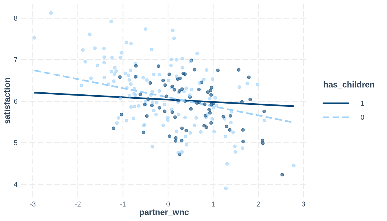

Partner WNC effect on satisfaction, by presence of children. The negative slope is flatter for couples with children.

SEM specification (wide format)

The SEM analogue creates manual product indicators in the wide data and fits a wide-format model with the products included.

Code

ddw$wnc_a_children <- ddw$wnc_a * ddw$has_children
ddw$wnc_p_children <- ddw$wnc_p * ddw$has_children

Code

model_sem_mod <- '
  # Actor (male) paths
  satisfaction_a ~ a*wnc_a + p*wnc_p + ar*recovery_a + pr*recovery_p +
    c*has_children + d*dual_earner +
    a_int*wnc_a_children + p_int*wnc_p_children

  # Partner (female) paths
  satisfaction_p ~ a*wnc_p + p*wnc_a + ar*recovery_p + pr*recovery_a +
    c*has_children + d*dual_earner +
    a_int*wnc_p_children + p_int*wnc_a_children

  # Intercepts (equal)
  satisfaction_a ~ int*1
  satisfaction_p ~ int*1

  # Residual variances (equal)
  satisfaction_a ~~ var*satisfaction_a
  satisfaction_p ~~ var*satisfaction_p

  # Predictor variances and covariances
  wnc_a ~~ wnc_p
  recovery_a ~~ recovery_p

  # Residual covariance
  satisfaction_a ~~ res_cov*satisfaction_p

  # --------------------------------------------------------
  # SIMPLE SLOPES (Calculated Parameters)
  # --------------------------------------------------------
  actor_slope_no_child   := a + a_int * 0
  actor_slope_has_child  := a + a_int * 1
  partner_slope_no_child  := p + p_int * 0
  partner_slope_has_child := p + p_int * 1
'

fit_sem_mod <- sem(model_sem_mod, data = ddw)
summary(fit_sem_mod, standardized = TRUE, fit.measures = TRUE)

lavaan 0.6-21 ended normally after 30 iterations

  Estimator                                         ML
  Optimization method                           NLMINB
  Number of model parameters                        31
  Number of equality constraints                    10

  Number of observations                           100

Model Test User Model:
                                                      
  Test statistic                               133.699
  Degrees of freedom                                30
  P-value (Chi-square)                           0.000

Model Test Baseline Model:

  Test statistic                               359.107
  Degrees of freedom                                39
  P-value                                        0.000

User Model versus Baseline Model:

  Comparative Fit Index (CFI)                    0.676
  Tucker-Lewis Index (TLI)                       0.579

Loglikelihood and Information Criteria:

  Loglikelihood user model (H0)               -654.118
  Loglikelihood unrestricted model (H1)       -587.268
                                                      
  Akaike (AIC)                                1350.236
  Bayesian (BIC)                              1404.945
  Sample-size adjusted Bayesian (SABIC)       1338.621

Root Mean Square Error of Approximation:

  RMSEA                                          0.186
  90 Percent confidence interval - lower         0.154
  90 Percent confidence interval - upper         0.219
  P-value H_0: RMSEA <= 0.050                    0.000
  P-value H_0: RMSEA >= 0.080                    1.000

Standardized Root Mean Square Residual:

  SRMR                                           0.193

Parameter Estimates:

  Standard errors                             Standard
  Information                                 Expected
  Information saturated (h1) model          Structured

Regressions:
                   Estimate  Std.Err  z-value  P(>|z|)   Std.lv  Std.all
  satisfaction_a ~                                                      
    wnc_a      (a)   -0.275    0.036   -7.535    0.000   -0.275   -0.403
    wnc_p      (p)   -0.218    0.036   -5.985    0.000   -0.218   -0.295
    recvry_   (ar)    0.233    0.035    6.576    0.000    0.233    0.296
    rcvry_p   (pr)    0.132    0.035    3.730    0.000    0.132    0.179
    hs_chld    (c)   -0.067    0.082   -0.816    0.414   -0.067   -0.046
    dul_rnr    (d)    0.284    0.074    3.860    0.000    0.284    0.186
    wnc__ch (a_nt)    0.095    0.069    1.383    0.167    0.095    0.084
    wnc_p_c (p_nt)    0.161    0.069    2.347    0.019    0.161    0.102
  satisfaction_p ~                                                      
    wnc_p      (a)   -0.275    0.036   -7.535    0.000   -0.275   -0.371
    wnc_a      (p)   -0.218    0.036   -5.985    0.000   -0.218   -0.320
    rcvry_p   (ar)    0.233    0.035    6.576    0.000    0.233    0.315
    recvry_   (pr)    0.132    0.035    3.730    0.000    0.132    0.168
    hs_chld    (c)   -0.067    0.082   -0.816    0.414   -0.067   -0.046
    dul_rnr    (d)    0.284    0.074    3.860    0.000    0.284    0.186
    wnc_p_c (a_nt)    0.095    0.069    1.383    0.167    0.095    0.060
    wnc__ch (p_nt)    0.161    0.069    2.347    0.019    0.161    0.142

Covariances:
                    Estimate  Std.Err  z-value  P(>|z|)   Std.lv  Std.all
  wnc_a ~~                                                               
    wnc_p              0.516    0.110    4.682    0.000    0.516    0.530
  recovery_a ~~                                                          
    rcvry_p            0.218    0.087    2.502    0.012    0.218    0.258
 .satisfaction_a ~~                                                      
   .stsfct_ (rs_c)     0.020    0.021    0.945    0.345    0.020    0.095

Intercepts:
                   Estimate  Std.Err  z-value  P(>|z|)   Std.lv  Std.all
   .stsfctn_ (int)    4.787    0.159   30.093    0.000    4.787    6.834
   .stsfctn_ (int)    4.787    0.159   30.093    0.000    4.787    6.827
    wnc_a             0.247    0.103    2.397    0.017    0.247    0.240
    wnc_p            -0.033    0.095   -0.353    0.724   -0.033   -0.035
    recovry_          3.005    0.089   33.684    0.000    3.005    3.368
    recvry_p          3.235    0.095   34.131    0.000    3.235    3.413

Variances:
                   Estimate  Std.Err  z-value  P(>|z|)   Std.lv  Std.all
   .stsfctn_ (var)    0.207    0.021    9.955    0.000    0.207    0.422
   .stsfctn_ (var)    0.207    0.021    9.955    0.000    0.207    0.421
    wnc_a             1.058    0.150    7.071    0.000    1.058    1.000
    wnc_p             0.896    0.127    7.071    0.000    0.896    1.000
    recovry_          0.796    0.113    7.071    0.000    0.796    1.000
    recvry_p          0.898    0.127    7.071    0.000    0.898    1.000

Defined Parameters:
                   Estimate  Std.Err  z-value  P(>|z|)   Std.lv  Std.all
    actr_slp_n_chl   -0.275    0.036   -7.535    0.000   -0.275   -0.403
    actr_slp_hs_ch   -0.179    0.076   -2.363    0.018   -0.179   -0.319
    prtnr_slp_n_ch   -0.218    0.036   -5.985    0.000   -0.218   -0.295
    prtnr_slp_hs_c   -0.057    0.076   -0.747    0.455   -0.057   -0.192

Compare MLM and SEM

The MLM and SEM should agree on the interaction coefficients (p_int in SEM ≈ partner_wnc:has_children in MLM). The differences will be in the standard errors (Wald in SEM vs. profile in MLM).

Code

# MLM partner-wnc × children
cat("MLM partner_wnc:has_children:\n")

MLM partner_wnc:has_children:

Code

cat("  estimate =", round(fixef(model_mod)["partner_wnc:has_children"], 4), "\n")

  estimate = 0.1613

Code

# SEM p_int
pe <- parameterEstimates(fit_sem_mod)
sem_p_int <- pe[pe$label == "p_int", "est"]
cat("SEM p_int:\n")

SEM p_int:

Code

cat("  estimate =", round(sem_p_int, 4), "\n")

  estimate = 0.1613 0.1613

What to take away

Key takeaways

A moderated APIM tests whether a dyad-level variable shapes actor or partner effects. The most common form: does the partner crossover effect vary by some dyad-level moderator?
In lme4, the moderation is a direct interaction term in the lmer formula. In lavaan, it is a manual product indicator in the wide-format data.
The two approaches give nearly identical point estimates.
Simple slopes and visualisations are the recommended way to report the conditional effects.

Setup

MLM specification

Likelihood ratio test

Simple slopes

Substantive interpretation

Visualise the interaction

SEM specification (wide format)

Compare MLM and SEM

What to take away

Key takeaways

What to read next